43 excel scatter diagram with labels
support.google.com › docs › answerAdd & edit a chart or graph - Computer - Google Docs Editors Help You can move some chart labels like the legend, titles, and individual data labels. You can't move labels on a pie chart or any parts of a chart that show data, like an axis or a bar in a bar chart. To move items: To move an item to a new position, double-click the item on the chart you want to move. Then, click and drag the item to a new position. How to Make a Scatter Plot in Excel | GoSkills Step 1: Organize your data. Ensure that your data is in the correct format. Since scatter graphs are meant to show how two numeric values are related to each other, they should both be displayed in two separate columns. The first column will usually be plotted on the X-axis and the second column on the Y-axis.
Scatter Diagram Help - BPI Consulting If you do, the program will add these as the labels for the X axis and Y axis. 2. Select "Scatter" from the "Cause and Effect" panel on the SPC for Excel ribbon. 3. The input screen for the scatter diagram is displayed. The program sets the initial X and Y ranges as the range that is selected on the worksheet.

Excel scatter diagram with labels
How to Create a Quadrant Chart in Excel – Automate Excel We’re almost done. It’s time to add the data labels to the chart. Right-click any data marker (any dot) and click “Add Data Labels.” Step #10: Replace the default data labels with custom ones. Link the dots on the chart to the corresponding marketing channel names. To do that, right-click on any label and select “Format Data Labels.” How to Create Scatter Plot In Excel - Career Karma It is easy to make a scatter plot in Excel when following a step-by-step guide. 1. Input Data and Organize Variables. The first thing you need to do is input the numerical values you will use in Excel and name your variables. Your first column would be your X-axis, and the second column would be the Y-axis value. How to Create Venn Diagram in Excel – Free Template Download By the end of this step-by-step tutorial, you will learn how build a dynamic Venn diagram in Excel completely from the ground up. Start Here; VBA. VBA Tutorial . Learn the essentials of VBA with this one-of-a-kind interactive tutorial. VBA Code Generator. Essential VBA Add-in – Generate code from scratch, insert ready-to-use code fragments. VBA Code Examples. 100+ VBA code …
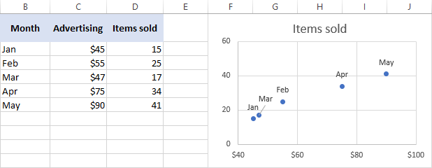
Excel scatter diagram with labels. How to Make a Scatter Plot in Excel with Two Sets of Data? To get started with the Scatter Plot in Excel, follow the steps below: Open your Excel desktop application. Open the worksheet and click the Insert button to access the My Apps option. Click the My Apps button and click the See All button to view ChartExpo, among other add-ins. The Problem With Labelling the Data Points in an Excel Scatter Chart The value of the X axis (the Run Time value in the above example). The value of the Y axis (the Budget value in the above example). The name of the data series (the word "Budget" in the above example). Identify which data point represents which film and then manually type in the film title. Seriously! Improve your X Y Scatter Chart with custom data labels Select the x y scatter chart. Press Alt+F8 to view a list of macros available. Select "AddDataLabels". Press with left mouse button on "Run" button. Select the custom data labels you want to assign to your chart. Make sure you select as many cells as there are data points in your chart. Press with left mouse button on OK button. Back to top Find, label and highlight a certain data point in Excel scatter graph 10.10.2018 · As the result, you will have a scatter plot with the average point labeled and highlighted: That's how you can spot and highlight a certain data point on a scatter diagram. To have a closer look at our examples, you are welcome to download our sample Excel Scatter Plot workbook. I thank you for reading and hope to see you on our blog next week.
Excel scatter chart using text name - Access-Excel.Tips Since Excel allows different chart types to be displayed in one chart, we are going to create a mix of bar chart (column chart) and scatter chart. Scatter chart is used to display the actual data point, while bar chart is to display Grade labels. - Create scatter chart for Range B20:C31 (Series 1) How to Create Dot Plots in Excel? - EDUCBA In this article, we will see how we can create the dot chart in excel. Though we have conventional scatter plots added under Excel, those can not be considered as dot plots. Example of Dot Plots in Excel. Suppose we have month-wise sales values for four different years, 2016, 2017, 2018 and 2019, respectively. We wanted to draw a dot plot based ... Scatter Graph - Overlapping Data Labels - Excel Help Forum The use of unrepresentative data is very frustrating and can lead to long delays in reaching a solution. 2. Make sure that your desired solution is also shown (mock up the results manually). 3. Make sure that all confidential data is removed or replaced with dummy data first (e.g. names, addresses, E-mails, etc.). 4. support.microsoft.com › en-us › officeAvailable chart types in Office - support.microsoft.com Scatter charts are typically used for displaying and comparing numeric values, such as scientific, statistical, and engineering data. Scatter charts have the following chart subtypes: Scatter chart with markers only Compares pairs of values. Use a scatter chart with data markers but without lines if you have many data points and connecting ...
Hover labels on scatterplot points - Excel Help Forum Hi Everyone, I am hoping someone can point me in the right direction on a challenge I am trying to solve. I have data on an xy scatterplot and would like to be able to move by mouse over the points and have a label show up for each point showing the X,Y value of the point and also text from a comment cell. I know excel has these hover labels but i cant seem to find a way to edit them. › charts › quadrant-templateHow to Create a Quadrant Chart in Excel – Automate Excel Step #9: Add the default data labels. We’re almost done. It’s time to add the data labels to the chart. Right-click any data marker (any dot) and click “Add Data Labels.” Step #10: Replace the default data labels with custom ones. Link the dots on the chart to the corresponding marketing channel names. Excel Scatter Chart with Labels - Super User Move the button down and out of the way of your data if you have more than a few columns. Paste your data in on top of the film data. Create scatter plots by selecting two column at a time and insert scatter (plot). Clicking on the button, which will add labels. Easy. How to Create a Sankey Diagram in Excel Spreadsheet Components of a Sankey Diagram in Excel. A Sankey is a minimalist diagram that consists of the following: Nodes: This is an element linked by “Flows.” Furthermore, it represents the events in each path. Flows: Flows link the nodes. And each flow is specified by the names of its source and target nodes in the “from” and “to” fields ...
3d scatter plot for MS Excel
Add Custom Labels to x-y Scatter plot in Excel Step 1: Select the Data, INSERT -> Recommended Charts -> Scatter chart (3 rd chart will be scatter chart) Let the... Step 2: Click the + symbol and add data labels by clicking it as shown below Step 3: Now we need to add the flavor names to the label. Now right click on the label and click format ...

Advanced Graphs Using Excel : create structure plot using excel
Available chart types in Office - support.microsoft.com When you create a chart in an Excel worksheet, a Word document, or a PowerPoint presentation, you have a lot of options. Whether you’ll use a chart that’s recommended for your data, one that you’ll pick from the list of all charts, or one from our selection of chart templates, it might help to know a little more about each type of chart.. Click here to start creating a chart.
Scatter Chart Examples
Add labels to scatter graph - Excel 2007 | MrExcel Message Board Nov 10, 2008. #1. OK, so I have three columns, one is text and is a 'label' the other two are both figures. I want to do a scatter plot of the two data columns against each other - this is simple. However, I now want to add a data label to each point which reflects that of the first column - i.e. I don't simply want the numerical value or ...

Creating 3-D Scatter Plots - MATLAB & Simulink - MathWorks América Latina
excel - How to label scatterplot points by name? - Stack Overflow This is what you want to do in a scatter plot: right click on your data point select "Format Data Labels" (note you may have to add data labels first) put a check mark in "Values from Cells" click on "select range" and select your range of labels you want on the points
Excel 2013 - Manually adding multiple data sets to scatter plot - YouTube
Scatter Plot Chart in Excel (Examples) | How To Create Scatter ... - EDUCBA Step 1: Select the data. Step 2: Go to Insert > Chart > Scatter Chart > Click on the first chart. Step 3: This will create the scatter diagram. Step 4: Add the axis titles, increase the size of the bubble and Change the chart title as we have discussed in the above example. Step 5: We can add a trend line to it.
How to make a scatter plot in Excel
ppcexpo.com › blog › sankeHow to Create a Sankey Diagram in Excel Spreadsheet Components of a Sankey Diagram in Excel. A Sankey is a minimalist diagram that consists of the following: Nodes: This is an element linked by “Flows.” Furthermore, it represents the events in each path. Flows: Flows link the nodes. And each flow is specified by the names of its source and target nodes in the “from” and “to” fields.

Excel - Scatter Chart Axis Labels | Overclockers UK Forums
› charts › venn-diagramHow to Create Venn Diagram in Excel – Free Template Download First, let’s add data labels. Right-click on the data marker representing Series “Pepsi” and choose “Add Data Labels.” Step #15: Customize data labels. Replace the default values with the custom labels you previously designed. Right-click on any data label and choose “Format Data Labels.” Once the task pane pops up, do the following:
Excel Scatterplot with Custom Annotation - PolicyViz
How to use a macro to add labels to data points in an xy scatter chart ... Click Chart on the Insert menu. In the Chart Wizard - Step 1 of 4 - Chart Type dialog box, click the Standard Types tab. Under Chart type, click XY (Scatter), and then click Next. In the Chart Wizard - Step 2 of 4 - Chart Source Data dialog box, click the Data Range tab.
Post a Comment for "43 excel scatter diagram with labels"